Preprocessing for the Adult Dataset

An incredibly important aspect of producing accurate machine learning models is the structure of the database the model is trained on. There are various ways we can manipulate the features (columns of the database) in ways that may positively (or negatively!) affect the performance of a model. This post will be about preprocessing a database.

In the previous ML project I covered, we were looking at the fundamentals of testing multiple algorithms on our data and how we can score them against one another. Today we’ll be doing a simpler version of that, while focusing mainly on the preprocessing we are applying to the dataset.

Preprocessing the Adult Dataset using pandas (photo by Mathias Appel)

The Adult Dataset

I’ve picked the adult dataset from the UCI Machine Learning Repository because it is incredibly popular so there’s a lot of help that exists for it, it has some missing values to deal with, and also because it has a lot of categorical variables.

By default, it is already separated into a test set and a validation set, so we will need to load both of these files and process them individually.

If you want to follow along then make sure to download your own copy of the datasets.

Let’s start off by reading the data with pandas:

import pandas as pd
import os

if __name__ == '__main__':
  filepathTrain = os.path.join(os.getcwd(), "Data/adult.data")
  filepathTest = os.path.join(os.getcwd(), "Data/adult.test")
  columns = ['age', 'workclass', 'fnlwgt', 'education', 'education-num', 'marital-status', 'occupation', 'relationship', 'race','sex', 'capital-gain', 'capital-loss', 'hours-per-week', 'native-country', 'salary']
  datasetTrain = pd.read_csv(filepathTrain, names = columns)
  datasetTest = pd.read_csv(filepathTest, names = columns)

Here I’m using the ‘os’ library to access the file-paths of my datasets, and then I’m manually entering all the column names, which I gathered from the UCI ML Repository webpage.

Note that I’m just going to be looking at the training set here (for clarity), but I highly recommend repeating all the following functions on the test set too!

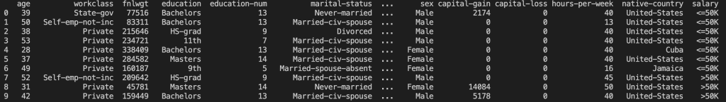
Now that we’ve loaded the data, let’s have a peak at the first ten lines:

print(datasetTrain.head(10))

Outputs:

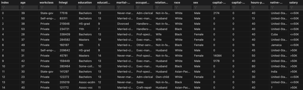
Note that this set has more features than pandas is willing to display by default. I want to have a look at all the feature columns so I’m going to use the data viewer in Visual Studio Code (my code environment). For details on how to do this, set a breakpoint after you’ve loaded the dataset and then hit the ‘run and debug’ button. In the ‘variables’ tab right click the ‘datasetTrain’ variable and click ‘View Value in Data Viewer’. This will open a tab for viewing the whole set:

Alternatively, if you are not working in Visual Studio Code, you could instead simply write:

pd.set_option('display.max_columns', None)
print(datasetTrain.head(10))

In any case, we get to see the first few lines of the set and can clearly see the structure.

Initial Dataset Analysis

For analysing the dataset I have decided to concatenate together the train and test sets that we have. This allows us to gain a more complete look at the data we have available to us. I’ll get more into the preprocessing in the following section but basically I’ve dropped any rows that contained a missing value and then added the test set to the bottom of the training set.

import pandas as pd
import os
import numpy as np

def ReplaceQsMarkWithNaN (data):
  return data.replace(to_replace = ' ?', value = np.nan)

if __name__ == '__main__':
  # Load Dataset
  filepathTrain = os.path.join(os.getcwd(), "Data/adult.data")
  filepathTest = os.path.join(os.getcwd(), "Data/adult.test")
  columns = ['age', 'workclass', 'fnlwgt', 'education', 'education-num', 'marital-status', 'occupation', 'relationship', 'race','sex', 'capital-gain', 'capital-loss', 'hours-per-week', 'native-country', 'salary']
  datasetTrain = pd.read_csv(filepathTrain, names = columns)
  datasetTest = pd.read_csv(filepathTest, names = columns)

  # Replace ' ?' values with NaN
  datasetTrain = ReplaceQsMarkWithNaN(datasetTrain)
  datasetTest = ReplaceQsMarkWithNaN(datasetTest)
   
  # Drop any row with a missing value
  datasetTrain = datasetTrain.dropna()
  datasetTest = datasetTest.dropna()

  # 'datasetTest' salary values have a full-stop in for no reason so this removes that
  datasetTest = datasetTest.replace(to_replace={' <=50K.': ' <=50K', ' >50K.':' >50K'})
   
  # For some reason the data types of 'datasetTest' were different so this sets it the same as 'datasetTrain'
  datasetTest = pd.DataFrame(datasetTest, columns=datasetTest.columns).astype(datasetTrain.dtypes.to_dict())

  # Concatenate the two sets together
  fullDataset = pd.concat([datasetTrain, datasetTest], axis = 0)

We can check the dimensions of the set:

...
print(fullDataset.shape)

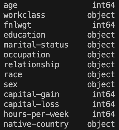
Next I would like to check the data-types of each column:

...
print(fullDataset.dtypes)

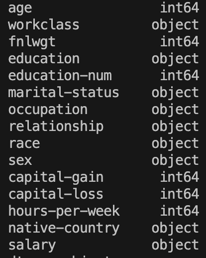
In terms of datatypes, we see a lot of columns have the datatype ‘object’. This tells us that these columns are categorical variables. We’ll discuss these in more depth later but a categorical variable usually takes string values to represent different items in a category. For example, the categorical variable ‘native-country’ takes values of ‘United-States’, ‘Cuba’, ‘India’,…. It’s important to identify columns like this because often machine learning algorithms are optimised to work only on numerical data, so they will throw errors if we feed in these categorical variables directly.

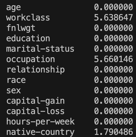
We can look in more detail at the numerical features:

...
print(fullDataset.describe())

Note that the ‘.describe()’ method will only show information related to numerical data, hence it only shows six columns. Let’s plot these as histograms:

from matplotlib import pyplot
...
fullDataset.hist(bins = 20)
pyplot.tight_layout()
pyplot.show()

Some things we notice are that ‘hours-per-week’ and ‘education-num’ may loosely resemble Gaussian distributions. Another is that ‘capital-gain’ and ‘capital-loss’ appear incredibly skewed – this is effectively confirmed by the quartile data and the standard deviation shown above. Perhaps we could apply some logarithmic transformation to these? Another thing worth noting is that ‘age’ and ‘fnlwgt’ seem to resemble exponential distributions. And finally, we should not ignore the x-axis scales – they differ enormously from one another and heavily suggest we should be scaling/normalising our numeric data.

Now let’s check the class distribution. I’m going to plot it as a pie chart:

...
labels = list(fullDataset.groupby('salary').size().index)
values = list(fullDataset.groupby('salary').size().values)

fig1, ax1 = pyplot.subplots()
ax1.pie(values, labels=labels, autopct='%1.1f%%', startangle = 180)
ax1.axis('equal')
pyplot.title('Proportion Of The Two Classes')
pyplot.show()

Here we can see we have imbalanced classes – there are far more instances of '<=50K' than ‘>50K’ in the set. This is important to know because it can influence which metric we choose to use for evaluating model performance later on.

The final thing I want to check is the ‘education-num’ column. I concatenated together the ‘education’ and ‘education-num’ column (separated by a ‘ – ‘) and then printed the unique values that appear in the resulting column:

...
concatEduCols = fullDataset['education'] + ' - ' + fullDataset['education-num'].astype(str)
print(pd.Series(concatEduCols.unique()))

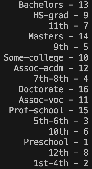
This shows us that the numbers in ‘education-num’ form a one-to-one correspondence with the labels in ‘education’. There is no reason to have both columns therefore I will choose to drop ‘education-num’.

Loading the Data

In this section we’re going to be writing a function to load all the data and do some basic operations on it.

We’ll start with just reading in the data, as we did before:

def LoadDataset(filepathTrain, filepathTest):
  # Read the data
  columns = ['age', 'workclass', 'fnlwgt', 'education', 'education-num', 'marital-status', 'occupation', 'relationship', 'race','sex', 'capital-gain', 'capital-loss', 'hours-per-week', 'native-country', 'salary']
  datasetTrain = pd.read_csv(filepathTrain, names = columns)
  datasetTest = pd.read_csv(filepathTest, names = columns)

Next I want to see if there’s anything we need to do with missing values. Information on the webpage for this set indicates clearly that there are missing values, however the following code seems to imply there aren’t missing values:

print(datasetTrain.isnull().sum())

It returns the sum of missing values in each column, yet returns 0 for all. Something is awry. I spent a while trying to figure out how my code was wrong but eventually found the answer, and learnt an important lesson. This code looks for missing values by finding cells containing ‘NaN’. However, this dataset has been prepared in a format where missing values are represented by a different character. To find this character, the technique I used was to simply print out random samples (of size 50) of the set until I found it:

...
sample = datasetTrain.sample(50)
print(sample)

Here’s an example sample:

Here, if you look closely, we can see the culprit! The character ‘?’ is used to represent missing values… or is it? If we highlight one of these cells by clicking it and selecting the text we see this:

So actually the character ‘ ?’ represents missing values (the white-space is critical to include). I spent way too long wondering why I couldn’t access the missing values with ‘?’.

Anyway, if we now do a find-and-replace with pandas, we can swap all the instances of ‘ ?’ to ‘NaN’, allowing us to use ‘isnull()’ to find missing values.

I will write a small function to do this task:

def ReplaceQsMarkWithNaN (data):
  return data.replace(to_replace = ' ?', value = np.nan)

Now we need to call this on our datasets:

...
datasetTrain = ReplaceQsMarkWithNaN(datasetTrain)
datasetTest = ReplaceQsMarkWithNaN(datasetTest)

print(datasetTrain.isnull().sum())

And this outputs:

Fantastic! Missing values are now appropriately formatted.

I mentioned above wanting to remove the ‘education-num’ column so let’s handle that next:

...
datasetTrain.drop('education-num', axis = 1, inplace=True)
datasetTest.drop('education-num', axis = 1, inplace=True)

Another thing I noticed is if we print the first few lines of ‘datasetTest’, we see this:

The first line here is clearly an error of some kind so I will be dropping it. This code will do the job:

...
datasetTest.drop(datasetTest.index[0], inplace=True)

Next we will split away the target variable (the ‘salary’ column) from the rest of the features:

...
XTrain = datasetTrain.drop('salary', axis = 1)
yTrain = datasetTrain['salary']

XTest = datasetTest.drop('salary', axis = 1)
yTest = datasetTest['salary']

If we check the unique values that exist in ‘yTrain’ and ‘yTest’ we expect that they will take the same values but that turns out to not be the case:

...
print(yTrain.unique())
print(yTest.unique())

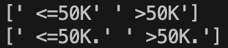
Someone decided they would add a full-stop into the values of ‘yTest’! We need to remove that; I’ll use pandas ‘.replace’:

yTest = yTest.replace(to_replace={' <=50K.': ' <=50K', ' >50K.':' >50K'})

Having done that I think we’re good to go! Here is the full function for loading and cleaning our data:

def LoadDataset(filepathTrain, filepathTest):
  # Read the data
  columns = ['age', 'workclass', 'fnlwgt', 'education', 'education-num', 'marital-status', 'occupation', 'relationship', 'race','sex', 'capital-gain', 'capital-loss', 'hours-per-week', 'native-country', 'salary']
  datasetTrain = pd.read_csv(filepathTrain, names = columns)
  datasetTest = pd.read_csv(filepathTest, names = columns)

  # Replace ? with NaN
  datasetTrain = ReplaceQsMarkWithNaN(datasetTrain)
  datasetTest = ReplaceQsMarkWithNaN(datasetTest)

  datasetTrain.drop('education-num', axis = 1, inplace=True)
  datasetTest.drop('education-num', axis = 1, inplace=True)

  # Drop first row of test set
  datasetTest.drop(datasetTest.index[0], inplace=True)

  # Split target feature away from the others
  XTrain = datasetTrain.drop('salary', axis = 1)
  yTrain = datasetTrain['salary']

  XTest = datasetTest.drop('salary', axis = 1)
  yTest = datasetTest['salary']

  # Remove full-stops in 'yTest'
  yTest = yTest.replace(to_replace={' <=50K.': ' <=50K', ' >50K.':' >50K'})

  return XTrain, yTrain, XTest, yTest

Missing Values

We’ve already seen that our data contains missing values. I’m going to discuss a couple of techniques we can use to deal with them. But before that, I want to see what kind of proportion of the data is missing. Here is a function that calculates the percentage of missing values per column:

def GetPercentageOfNaNValuesPerColumn (data):
  totalCount = data.count()
  NaNCount = data.isnull().sum()
  return 100*NaNCount / (totalCount + NaNCount)

Then we can call it as follows:

if __name__ == '__main__':
  # Load Dataset
  filepathTrain = os.path.join(os.getcwd(), "Data/adult.data")
  filepathTest = os.path.join(os.getcwd(), "Data/adult.test")
   
  XTrain, yTrain, XTest, yTest = LoadDataset(filepathTrain, filepathTest)

  print(GetPercentageOfNaNValuesPerColumn(XTrain))

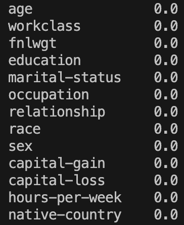
And this outputs:

This shows that we never have more than about 6% of the data missing in a column. So what can we do about this?

These are the methods I will discuss:

• Dropping columns with missing values
• Dropping rows with missing values
• Imputing

Drop the Columns or Rows

The simplest method is to simply drop a column if it has any missing values. The risk with this is that we will lose potentially valuable data that could improve the accuracy of the model. So this approach is only really worthwhile if a large proportion of the column is missing. If 40%, say, of a column is missing values then the best approach may be to drop it. Of course this depends on the importance of the column to the model, but with a high proportion of missing values it generally won’t be usable.

In our case, we only have ~6% missing values so we would be wasting a lot of data if we just dropped these columns.

Alternatively we could drop the rows which have missing values. Recall that I did this when doing the data visualisation above, so we can see how many rows were removed by doing that.

This is a before and after of the shape of ‘datasetTrain’:

And this is the equivalent for ‘datasetTest’:

So over the two sets we lose 3621 rows or about 7% of the total rows. I think this is a perfectly valid approach to use in this case.

Imputing Values

Imputing values is all about how we can attempt to fill the missing values using the other data in that column. There are various imputing strategies we can use. Some simple versions include using mean, median, most frequent, etc…. For example, the mean strategy will calculate the mean of all the numbers that we do have in the column, and will then substitute that value in place of any ‘NaN’ values.

There are more advanced methods like KNN, Moving Average, MICE, etc. but we won’t concern ourselves with these yet.

This approach is good because we don’t lose any data, however the risk is that we are inserting data that isn’t necessarily a real observation so it could skew how our model performs. For small proportions of missing values, imputation is usually a good option. It is what I will be using for this project.

One extension to just imputing values is to add another column to the dataset that acts as a flag to indicate whether data in that row has been imputed or not. Then the model is able to take imputed data less seriously. I won’t be doing this but it’s worth knowing about the method.

Let’s implement an imputer!

The sklearn library contains a class called ‘SimpleImputer’ that we can use. We want to import the SimpleImputer class and then apply it to our data. Because the only missing values in our set are in columns of non-numerical data, we will need to fill the values using the ‘most_frequent’, or the mode, of that column.

We can set up our imputer as follows:

from sklearn.impute import SimpleImputer
...
imputer = SimpleImputer(strategy='most_frequent')

We need to first ‘fit’ the imputer to the values of the ‘XTrain’ set. This basically just means that it will figure out what the most frequent value in each column is (because our imputer strategy is ‘most_frequent’). Then we need to ‘transform’ the data using the imputer. This involves substituting in this previously calculated ‘most_frequent’ value to all missing values in the column. We can do both of these operations in one using the ‘fit_transform’ method.

...
imputer = SimpleImputer(strategy='most_frequent')
XTrainImputed = pd.DataFrame(imputer.fit_transform(XTrain))

Note that imputing returns a numpy array, so I’m converting the result back to a pandas ‘DataFrame’.

To apply the imputer to the test/validation set, we DON’T want to fit it again to that set’s values. We want to fill the missing cells in the test set using the previously calculated most-frequent values from the training set. This is an important point and easy to mess up. The reason why is that we aren’t allowed to use data from the test set (like its most-frequent value) for anything related to model training. The only data we can use and manipulate for the model is that which is in the training set. It’s kind of like training the model on some data, and then testing it on that same data. The results will not reflect real-world performance. For more information on this see data leakage.

So to apply the imputer to the test set, we don’t want to call ‘fit’ first, we just want to call ‘transform’:

...
imputer = SimpleImputer(strategy='most_frequent')
XTrainImputed = pd.DataFrame(imputer.fit_transform(XTrain))
XTestImputed = pd.DataFrame(imputer.transform(XTest))

This will now have filled all our missing values! But the new DataFrames created don’t have any of the column names anymore so I will add them back in:

...
XTrainImputed.columns = XTrain.columns
XTestImputed.columns = XTest.columns

Moreover, the imputer seems to have changed the data types of all columns to ‘object’. I believe this occurs when we use the ‘most_frequent’ strategy, especially since we have applied it to all columns (rather than just the ones with missing values). We can reinstate the old data types as follows:

...
XTrainImputed = pd.DataFrame(XTrainImputed, columns=XTrain.columns).astype(XTrain.dtypes.to_dict())
XTestImputed = pd.DataFrame(XTestImputed, columns=XTest.columns).astype(XTest.dtypes.to_dict())

Great so all our code together looks like this right now:

import pandas as pd
import os
import numpy as np
from sklearn.impute import SimpleImputer

def ReplaceQsMarkWithNaN (data):
  ...

def GetPercentageOfNaNValuesPerColumn (data):
  ...

def LoadDataset (filepathTrain, filepathTest):
  ...

if __name__ == '__main__':
  # Load Dataset
  filepathTrain = os.path.join(os.getcwd(), "Data/adult.data")
  filepathTest = os.path.join(os.getcwd(), "Data/adult.test")
   
  XTrain, yTrain, XTest, yTest = LoadDataset(filepathTrain, filepathTest)

  # Impute missing values
  imputer = SimpleImputer(strategy='most_frequent')
  XTrainImputed = pd.DataFrame(imputer.fit_transform(XTrain))
  XTestImputed = pd.DataFrame(imputer.transform(XTest))

  # Imputing removed column names; add them back
  XTrainImputed.columns = XTrain.columns
  XTestImputed.columns = XTest.columns

  # Imputing has made data type of all columns 'object'; reinstate the old data types
  XTrainImputed = pd.DataFrame(XTrainImputed, columns=XTrain.columns).astype(XTrain.dtypes.to_dict())
  XTestImputed = pd.DataFrame(XTestImputed, columns=XTest.columns).astype(XTest.dtypes.to_dict())

Just to make sure we’ve done everything correctly, let’s have a look at the proportions of missing values, the column names, and the data types of our dataset.

...
print(GetPercentageOfNaNValuesPerColumn(XTrainImputed))

Great! No missing values remain! The same is true for the test set (check that yourself however).

...
print(XTrainImputed.head())

Printing ‘.head()’ shows that we indeed have the correct column names.

...
print(XTrainImputed.dtypes)

Fantastic! Everything is as intended and we have no more missing values!

Categorical Variables

The other task we need to do before we can apply Machine Learning algorithms is to convert categorical variables into numerical values. To achieve this we need to encode the values the categorical variables take in some way. There exist two different types of categorical variable and this influences the methods we can use.

The different types of categorical variable are:

• Ordinal:
  • Ordinal categorical variables have a natural ordering to them.
  • For example, if we had a variable called ‘frequency’ that took values ‘never’, ‘rarely’, ‘sometimes’, ‘often’, ‘always’, then we can see a clear ordering for these values. We could assign the number 1 to ‘never’, 2 to ‘rarely’, and so on up to 5 for ‘always’. This method of encoding is called Ordinal Encoding.
• Nominal:
  • Nominal categorical variables do not have any natural order.
  • An example from our dataset is the ‘native-country’ variable. There is no natural order we can provide for the values ‘United-States’, ‘Thailand’, ‘Ireland’, etc.
  • In general, it is not recommended to use ordinal encoding on nominal variables. A different method we can use is called one-hot encoding.

You may wonder why we shouldn’t use ordinal encoding to just randomly assign numbers to each value of a nominal variable anyway. The reason is that if, for example, we assigned 1 to ‘United-States’ and 2 to ‘Thailand’ then, because there exists the mathematical relation 1 < 2, our machine learning algorithm might infer that somehow United-States is ‘less than’ Thailand. This may end up influencing how our model learns.

Let’s take a closer look at both ordinal encoding and one-hot encoding.

Ordinal Encoding

As I was saying before, ordinal encoding will perform better when applied to ordinal categorical variables – we don’t want to impose an ordering where none exists. It assigns a number to each unique value that the variable takes. Here’s an example of ordinal encoding applied to a column:

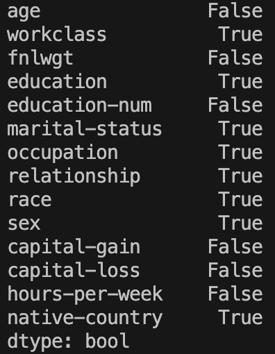
Let’s look at our categorical variables and see if any could be ordinal. Note that we can find the categorical variables by searching for columns which have data type ‘object’. I’m going to walk slowly through the code for getting this list because it’s not very intuitive. Firstly let’s produce a Series representing whether a column has data type ‘object’ or not:

...
categoricalColumns = (XTrainImputed.dtypes == 'object')

Printing this variable gives:

So we want to extract from this the ‘True’ values only. Note that in pandas we can index using boolean arrays. So the array [False, True, True] would access the 2nd and 3rd rows in a Series of size 3. We can use this here, by passing True to the rows with value True, and False to the rows with value False. A clever way to do this is to index the data series with itself!

...
categoricalColumns = (XTrainImputed.dtypes == 'object')
print(categoricalColumns[categoricalColumns])

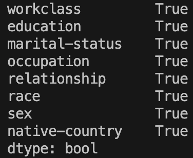
Great! The column labels at the side are the index of this series. We can access these by just adding ‘.index’. I also will convert the result to a standard Python list:

categoricalColumns = (XTrainImputed.dtypes == 'object')
categoricalColumns = list(categoricalColumns[categoricalColumns].index)
print(categoricalColumns)

And that’s our list of categorical variables. I will actually move this code into a function so we can use it again:

def GetCategoricalColumns (data):
  categoricalColumns = (data.dtypes == 'object')
  categoricalColumns = list(categoricalColumns[categoricalColumns].index)
  return categoricalColumns

So are any of these categorical variables appropriate for ordinal encoding? You can often tell by just reading the variable name, but to be safe I decided to print out each variable’s unique values in turn. For example, to do this for the ‘workclass’ column you would write:

print(XTrainImputed['workclass'].unique())

To my eye, this list appears nominal so ordinal encoding probably isn’t the way forward. Doing this to all categorical variables implies that just ‘education’ is ordinal. The ‘education’ unique values are as follows:

If you remember back when we were cleaning the dataset, I removed a column called ‘education-num’. That column actually held the ordinal encoding of the ‘education’ column but I wanted to do it myself. The ordering that column used was as follows: ‘Preschool’ < ‘1st-4th’ < ‘5th-6th’ < ‘7th-8th’ < ‘9th’ < ’10th’ < ’11th’ < ’12th’ < ‘HS-grad’ < ‘Some-college’ < ‘Assoc-voc’ < ‘Assoc-acdm’ < ‘Bachelors’ < ‘Masters’ < ‘Prof-school’ < ‘Doctorate’.

So let’s try and apply an Ordinal Encoder to the ‘education’ column.

First we want to write out the ordering I just described as a list (first element ‘Preschool’,…, last element ‘Doctorate’). We will be using the sklearn ‘OrdinalEncoder’ class so let’s create the object and give it this ordering:

ordinalEncodingOrder = [' Preschool', ' 1st-4th', ' 5th-6th', ' 7th-8th', ' 9th', ' 10th', ' 11th', ' 12th', ' HS-grad',' Some-college', ' Assoc-voc', ' Assoc-acdm', ' Bachelors', ' Masters', ' Prof-school', ' Doctorate']
ordinalEncoder = OrdinalEncoder(categories=[ordinalEncodingOrder])

If we didn’t provide a value for ‘categories’, the encoder would automatically create the order and it would probably not be as we intended. Also as another gotcha, notice the white space at the beginning of each string here. I don’t know why these strings have this space but it’s just the form the data came in so we have to include it (or we could have removed it when we were cleaning the set but it’s not necessary).

Now we can use this encoder to transform the data. It works similarly to the ‘SimpleImputer’ from before; we first ‘fit_transform’ the encoder on the training set, and then ‘transform’ the test set. Note that I also create a new copy of the data before doing this.

...
XTrainEncoded = XTrainImputed.copy()
XTestEncoded = XTestImputed.copy()

ordinalEncoder = OrdinalEncoder(categories=[ordinalEncodingOrder])
XTrainEncoded['education'] = ordinalEncoder.fit_transform(XTrainImputed.loc[:,['education']])
XTestEncoded['education'] = ordinalEncoder.transform(XTestImputed.loc[:,['education']])

Let’s see what this has done. I’ll print the first 15 lines before we encode this column, and then after we’ve encoded it:

So we can see that, for example, ‘Bachelors’ is now ‘12.0’, and ‘9th’ is now ‘4.0’, etc.

One-Hot Encoding

We have a few other categorical variables that we need to deal with but, since they are nominal variables, ordinal encoding doesn’t seem appropriate for them. As such, we might consider One-Hot Encoding.

This method involves creating a new column for each unique value a categorical variable can take. Then we use these new columns as flags for each value. This is done by leaving a 0 in every column that isn’t that correct value, and a 1 in the column which does represent the value. Here’s an example:

Clearly this method has potential to add hugely many additional columns to the dataset, so we might want to be careful before we do it. Generally it is inappropriate to apply to variables that have high cardinality (take many different unique values). It might be worth printing out the cardinality of each of our nominal variables to verify that one-hot encoding will be okay:

...
numUniqueCategorical = XTrainEncoded[GetCategoricalColumns(XTrainEncoded)].nunique()
print(numUniqueCategorical)

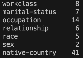
All of these seem fairly low cardinality except perhaps ‘native-country’. I feel as though 41 is quite high but I don’t think it’s high enough to warrant us not using one-hot encoding. But for reference, if we one-hot encode all of these columns we will end up with an additional 76 columns. So with 48842 rows total, we will be adding an additional 3,711,992 cells to the set. This sounds like a lot but machine learning algorithms are optimised to run on vast quantities of data so in practice this number is fine.

Let’s proceed with applying the One-Hot Encoding. This will be slightly harder than Ordinal Encoding because we need to remove the old columns entirely and add one new column for each possible value of each categorical variable. Most of this will be handled by the sklearn ‘OneHotEncoder’ class. Let’s begin by creating the ‘OneHotEncoder’ object and then using it to produce the additional columns we will add to the dataset:

from sklearn.preprocessing import OneHotEncoder
...
OHEncoder = OneHotEncoder(sparse=False)
onehotColumns = GetCategoricalColumns(XTrainEncoded)
XTrainOHCols = pd.DataFrame(OHEncoder.fit_transform(XTrainEncoded[onehotColumns]))
XTestOHCols = pd.DataFrame(OHEncoder.transform(XTestEncoded[onehotColumns]))

Note that we haven’t modified any of the dataset columns yet. We’ve produced new DataFrames containing only the new one-hot encodings of the appropriate columns. These new DataFrames don’t have any information regarding the index of the rows so let’s add that back in:

...
XTrainOHCols.index = XTrain.index
XTestOHCols.index = XTest.index

Then we want to drop the old categorical columns that we don’t need anymore, leaving us with just the numerical columns of the dataset. Let’s make a new DataFrame to hold just these numerical columns:

...
XTrainNumericalCols = XTrainEncoded.drop(onehotColumns, axis = 1)
XTestNumericalCols = XTestEncoded.drop(onehotColumns, axis = 1)

This doesn’t lose index information because we haven’t created a new DataFrame, just removed columns from the old one. Now we can form our One-Hot Encoded dataset by just concatenating the numerical columns with the one-hot encoded columns:

...
XTrainEncoded = pd.concat([XTrainOHCols, XTrainNumericalCols], axis = 1)
XTestEncoded = pd.concat([XTestOHCols, XTestNumericalCols], axis = 1)

This is all great except for two things. Let’s look at the shape of ‘XTestEncoded’ before and after doing the one-hot encoding:

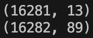
Note that we’ve gained the 76 columns we expected but we’re not supposed to gain any extra rows! Strangely this didn’t happen to ‘XTrainEncoded’. This apparently is an issue that can occur when performing multiple operations on a single DataFrame. Sometimes the index can persist in memory; the dimensions of the data can change but the indices don’t. In any case we can fix the issue by calling ‘.reset_index()’ on each of the sets we are concatenating to form ‘XTestEncoded’. So instead of the above we now have:

...
XTrainEncoded = pd.concat([XTrainOHCols, XTrainNumericalCols], axis = 1)
XTestEncoded = pd.concat([XTestOHCols.reset_index(drop=True), XTestNumericalCols.reset_index(drop=True)], axis = 1)

The final thing to fix stems from the fact that the column names of the new one-hot encoded variables are integers. Let’s print out a list of column names to see this:

We have the integers 0-82, mixed with some strings at the end. Some machine learning models don’t like this mix of ‘int’ and ‘str’ data types in column names so we better just convert them all to ‘str’:

...
XTrainEncoded.columns = XTrainEncoded.columns.astype(str)
XTestEncoded.columns = XTestEncoded.columns.astype(str)

Now we’re done! Here is all our code so far:

import pandas as pd
import os
import numpy as np
from sklearn.impute import SimpleImputer
from sklearn.preprocessing import OrdinalEncoder
from sklearn.preprocessing import OneHotEncoder

def ReplaceQsMarkWithNaN (data):
  ...

def GetPercentageOfNaNValuesPerColumn (data):
  ...

def GetCategoricalColumns (data):
  ...

def LoadDataset(filepathTrain, filepathTest):
  ...

if __name__ == '__main__':
  # Load Dataset
  filepathTrain = os.path.join(os.getcwd(), "Data/adult.data")
  filepathTest = os.path.join(os.getcwd(), "Data/adult.test")
   
  XTrain, yTrain, XTest, yTest = LoadDataset(filepathTrain, filepathTest)

  # Impute missing values
  imputer = SimpleImputer(strategy='most_frequent')
  XTrainImputed = pd.DataFrame(imputer.fit_transform(XTrain))
  XTestImputed = pd.DataFrame(imputer.transform(XTest))

  # Imputing removed column names; add them back
  XTrainImputed.columns = XTrain.columns
  XTestImputed.columns = XTest.columns

  # Imputing has made data type of all columns 'object'; reinstate the old data types
  XTrainImputed = pd.DataFrame(XTrainImputed, columns=XTrain.columns).astype(XTrain.dtypes.to_dict())
  XTestImputed = pd.DataFrame(XTestImputed, columns=XTest.columns).astype(XTest.dtypes.to_dict())

  # Ordinal encode the education column
  ordinalEncodingOrder = [' Preschool', ' 1st-4th', ' 5th-6th', ' 7th-8th', ' 9th', ' 10th', ' 11th', ' 12th', ' HS-grad',' Some-college', ' Assoc-voc', ' Assoc-acdm', ' Bachelors', ' Masters', ' Prof-school', ' Doctorate']
  ordinalEncoder = OrdinalEncoder(categories=[ordinalEncodingOrder])

  XTrainEncoded = XTrainImputed.copy()
  XTestEncoded = XTestImputed.copy()

  XTrainEncoded['education'] = ordinalEncoder.fit_transform(XTrainImputed.loc[:,['education']])
  XTestEncoded['education'] = ordinalEncoder.transform(XTestImputed.loc[:,['education']])

  # One-Hot Encode the columns
  OHEncoder = OneHotEncoder(sparse=False)
  onehotColumns = GetCategoricalColumns(XTrainEncoded)

  # Create new dataframe to hold OH encoded columns
  XTrainOHCols = pd.DataFrame(OHEncoder.fit_transform(XTrainEncoded[onehotColumns]))
  XTestOHCols = pd.DataFrame(OHEncoder.transform(XTestEncoded[onehotColumns]))
   
  # Put the index back in
  XTrainOHCols.index = XTrain.index
  XTestOHCols.index = XTest.index

  # Extract out the numerical columns
  XTrainNumericalCols = XTrainEncoded.drop(onehotColumns, axis = 1)
  XTestNumericalCols = XTestEncoded.drop(onehotColumns, axis = 1)
   
  # Concatenate the OH columns and the numerical columns to form complete encoded set
  XTrainEncoded = pd.concat([XTrainOHCols, XTrainNumericalCols], axis = 1)
  XTestEncoded = pd.concat([XTestOHCols.reset_index(drop=True), XTestNumericalCols.reset_index(drop=True)], axis = 1)

  # Set dtype of column names to string
  XTrainEncoded.columns = XTrainEncoded.columns.astype(str)
  XTestEncoded.columns = XTestEncoded.columns.astype(str)

Scaling Numeric Values

We’ve now successfully dealt with both our ordinal and nominal categorical variables but we haven’t looked at the numerical variables at all. Recall when we were looking at the histograms for these that I mentioned the scales looking very different from one another. This suggests that we should normalise the numeric variables to be within the range [0,1].

First we need a function that will find us all the numeric columns. We should be careful here because now that we’ve encoded all the categorical variables, every column appears numerical. If I repeated this project I would deal with numeric variables first. We’ll be okay though because we can still use the initial dataset, before we did any encoding, to find which columns are numeric. Here are the datatypes of the initial set (recalling that we’ve already removed the ‘education-num’ column):

So let’s write a function to access the columns of type ‘int64’. This follows similarly to the function we wrote to find columns of type ‘object’ so refer to that for an explanation:

def GetNumericalColumns(data):
  numColumns = (data.dtypes == 'int64')
  numColumns = list(numColumns[numColumns].index)
  return numColumns

Then calling the following will provide us with the correct columns:

...
numericColumns = GetNumericalColumns(XTrain)

To perform the scaling we will be using the ‘MinMaxScaler’ from sklearn. This needs to be ‘fit’ on the training set, which entails finding the smallest and largest values and figuring out what multiplier will send them to 0 and 1 respectively. Then we can ‘transform’ the set, scaling every other value by this multiplier to be within the range [0,1]. It’s a similar process to the imputer and encoders. We start by creating the object:

from sklearn.preprocessing import MinMaxScaler
...
scaler = MinMaxScaler()

Then we just need to apply it to the numeric columns we found earlier:

...
scaler = MinMaxScaler()
numericColumns = GetNumericalColumns(XTrain)
XTrainEncoded[numericColumns] = scaler.fit_transform(XTrainEncoded[numericColumns])
XTestEncoded[numericColumns] = scaler.transform(XTestEncoded[numericColumns])

Let’s check if it’s worked. Here are numeric columns before scaling:

Here are numeric columns after scaling:

They are indeed scaled! Great! Now every numeric and categorical column has been dealt with.

Encoding the Target Variable

The only thing left to do is encode the target variable – the salary column. The values our classes take are currently ‘<=50K’ and ‘>50K’. We can do label encoding to convert the classes to 0 and 1 respectively. Label encoding is essentially ordinal encoding but where the order doesn’t matter. It is intended to be used specifically for encoding the target variable in classification problems.

Using the label encoder works in the same way as the others so hopefully you can follow this code:

from sklearn.preprocessing import LabelEncoder
...
labelEnc = LabelEncoder()
   
yTrainEncoded = pd.Series(labelEnc.fit_transform(yTrain))
yTestEncoded = pd.Series(labelEnc.transform(yTest))

yTrainEncoded.index = yTrain.index
yTestEncoded.index = yTest.index

Now let’s print out the number of occurrences of each class in ‘yTrain’ before and after we’ve done the encoding:

So we can see that ‘<=50K’ has been mapped to 0 and ‘>50K’ has been mapped to 1, as intended.

At this point, we’ve encoded/scaled every variable. Now we can start looking at applying models!

Here is all the preprocessing code that we’ve written so far:

import pandas as pd
import os
import numpy as np
from sklearn.impute import SimpleImputer
from sklearn.preprocessing import OrdinalEncoder
from sklearn.preprocessing import OneHotEncoder
from sklearn.preprocessing import MinMaxScaler
from sklearn.preprocessing import LabelEncoder


def ReplaceQsMarkWithNaN (data):
  ...

def GetPercentageOfNaNValuesPerColumn (data):
  ...

def GetCategoricalColumns (data):
  ...

def GetNumericalColumns (data):
  ...

def LoadDataset (filepathTrain, filepathTest):
  ...

if __name__ == '__main__':
  # Load Dataset
  filepathTrain = os.path.join(os.getcwd(), "Data/adult.data")
  filepathTest = os.path.join(os.getcwd(), "Data/adult.test")
   
  XTrain, yTrain, XTest, yTest = LoadDataset(filepathTrain, filepathTest)

  # Impute missing values
  imputer = SimpleImputer(strategy='most_frequent')
  XTrainImputed = pd.DataFrame(imputer.fit_transform(XTrain))
  XTestImputed = pd.DataFrame(imputer.transform(XTest))

  # Imputing removed column names; add them back
  XTrainImputed.columns = XTrain.columns
  XTestImputed.columns = XTest.columns

  # Imputing has made data type of all columns 'object'; reinstate the old data types
  XTrainImputed = pd.DataFrame(XTrainImputed, columns=XTrain.columns).astype(XTrain.dtypes.to_dict())
  XTestImputed = pd.DataFrame(XTestImputed, columns=XTest.columns).astype(XTest.dtypes.to_dict())

  # Ordinal encode the education column
  ordinalEncodingOrder = [' Preschool', ' 1st-4th', ' 5th-6th', ' 7th-8th', ' 9th', ' 10th', ' 11th', ' 12th', ' HS-grad',' Some-college', ' Assoc-voc', ' Assoc-acdm', ' Bachelors', ' Masters', ' Prof-school', ' Doctorate']
  ordinalEncoder = OrdinalEncoder(categories=[ordinalEncodingOrder])

  XTrainEncoded = XTrainImputed.copy()
  XTestEncoded = XTestImputed.copy()

  XTrainEncoded['education'] = ordinalEncoder.fit_transform(XTrainImputed.loc[:,['education']])
  XTestEncoded['education'] = ordinalEncoder.transform(XTestImputed.loc[:,['education']])

  # One-Hot Encode the columns
  OHEncoder = OneHotEncoder(sparse=False)
  onehotColumns = GetCategoricalColumns(XTrainEncoded)

  # Create new dataframe to hold OH encoded columns
  XTrainOHCols = pd.DataFrame(OHEncoder.fit_transform(XTrainEncoded[onehotColumns]))
  XTestOHCols = pd.DataFrame(OHEncoder.transform(XTestEncoded[onehotColumns]))
   
  # Put the index back in
  XTrainOHCols.index = XTrain.index
  XTestOHCols.index = XTest.index

  # Extract out the numerical columns
  XTrainNumericalCols = XTrainEncoded.drop(onehotColumns, axis = 1)
  XTestNumericalCols = XTestEncoded.drop(onehotColumns, axis = 1)
   
  # Concatenate the OH columns and the numerical columns to form complete encoded set
  XTrainEncoded = pd.concat([XTrainOHCols, XTrainNumericalCols], axis = 1)
  XTestEncoded = pd.concat([XTestOHCols.reset_index(drop=True), XTestNumericalCols.reset_index(drop=True)], axis = 1)

  # Set dtype of column names to string
  XTrainEncoded.columns = XTrainEncoded.columns.astype(str)
  XTestEncoded.columns = XTestEncoded.columns.astype(str)

  # Scale numerical columns
  scaler = MinMaxScaler()
  numericColumns = GetNumericalColumns(XTrain)

  XTrainEncoded[numericColumns] = scaler.fit_transform(XTrainEncoded[numericColumns])
  XTestEncoded[numericColumns] = scaler.transform(XTestEncoded[numericColumns])

  # Encode the target variable
  labelEnc = LabelEncoder()

  yTrainEncoded = pd.Series(labelEnc.fit_transform(yTrain))
  yTestEncoded = pd.Series(labelEnc.transform(yTest))

  yTrainEncoded.index = yTrain.index
  yTestEncoded.index = yTest.index

Testing Models

In the last project we covered I spoke about using a cross-validation method to gain an accurate measure of how well a model performs over the training set. Today however, because we’ve done a lot of preprocessing and that is the main concept we’re focusing on, I will not be using cross-validation but simply a train/test split. You will have noticed the whole way through that our set is already split into ‘XTrain’ and ‘XTest’ so now we can finally make use of this.

I’ve picked out a variety of models of different types to test with:

• Ridge Classifier
• Logistic Regression
• Stochastic Gradient Descent
• K-Nearest Neighbours
• Linear Discriminant Analysis
• Gaussian Naive Bayes
• Decision Tree Classifier
• XGBoost Classifier

Let’s make a function to load all these models into a list:

...
from sklearn.linear_model import RidgeClassifier
from sklearn.linear_model import LogisticRegression
from sklearn.linear_model import SGDClassifier
from sklearn.neighbors import KNeighborsClassifier
from sklearn.discriminant_analysis import LinearDiscriminantAnalysis
from sklearn.naive_bayes import GaussianNB
from sklearn.tree import DecisionTreeClassifier
from xgboost import XGBClassifier
...
def CreateModels():
  models = []
  models.append(['RidgeClassifier', RidgeClassifier()])
  models.append(['LogisticRegression', LogisticRegression(solver='liblinear')])
  models.append(['SGD', SGDClassifier()])
  models.append(['KNN', KNeighborsClassifier()])
  models.append(['LDA', LinearDiscriminantAnalysis()])
  models.append(['GaussianNB', GaussianNB()])
  models.append(['Tree', DecisionTreeClassifier()])
  models.append(['XGB', XGBClassifier()])
  return models

Now we can call this to access our list of models, but then we want to loop through them to test the performance. Here is the loop I will be using:

...
models = CreateModels()

for name, model in models:
  model.fit(XTrainEncoded, yTrainEncoded)
  predictions = model.predict(XTestEncoded)
  print('%s: %.3f' % (name, accuracy_score(yTestEncoded, predictions)))

I want to discuss the fact that I’m using classification accuracy as a scoring metric. We saw earlier on that our dataset has imbalanced classes. We have to be careful using classification accuracy on a set like this because it can be very misleading. For example, if we had a binary classification problem with 99% of the classes being ‘0’ and 1% of classes being ‘1’, then a no-skill model that is just guessing ‘0’ for every prediction will achieve a 99% accuracy. This is useless and shows that we would need to turn to other metrics in this case.

For our dataset, the imbalance is not too severe and also the two classes carry equal importance so I believe we can get away with using classification accuracy. We just need to remember that ~75% of our classes are ‘<=50K’ so this will be the baseline – any model that achieves an accuracy of 75% or less does not have any skill.

Let’s run the tests for our models!

The results are as follows:

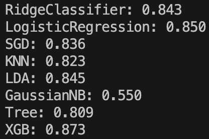
A model that stands out is the Gaussian Naive Bayes. It’s accuracy is at 55% – far lower than a no-skill model guessing ‘<=50K’ every time. I imagine the reason for this is because this model assumes a Gaussian distribution for each of our numerical inputs, however this is far from the truth as we saw when analysing the histograms. If anyone is able to explain in any more detail why the model has performed so badly I’d love to know!

Ignoring that, our top three performers are XGBoost, Logistic Regression, and Linear Discriminant Analysis.

Improving Results

At this point in a full project I would look to dive deeper into the top three performers that we have identified. I would try different algorithms that live in the same overall families as each of these three to try and find another good performer. I would then look to tune some of the parameters of the new top performers and hopefully squeeze out some additional improvements. Finally, it might be worth trying to combine a selection of the best models into some kind of ensemble model that benefits from each of their strengths whilst mitigating their weaknesses.

Since the focus for this project has been on preprocessing I will not concern myself with those steps here.

Conclusion

We’ve covered a lot about preprocessing with this project, including dataset preparation/cleaning, dealing with missing values, dealing with categorical variables, and scaling numeric features. I wanted to cover how to do all of these things ‘by hand’ since it’s my first attempt doing all of this on a dataset by myself. I’m aware that a far more efficient approach would be to use sklearn pipelines, and indeed I may publish a follow-up to this post which covers the same project but using pipelines instead.

In any case, we successfully managed to manipulate our data and get it into a form that allowed us to use machine learning algorithms. We ended up with a top performance of 87.3% classification accuracy, by XGBoost.

Here are some of the things I learnt while researching/writing this project:

• pandas requires that missing values are represented by ‘NaN’, however not all datasets are going to be formatted in this way so that needs to be checked straight away. You can print out random samples of the set to try to find the special character used – and check for white space in the value too!
• Some columns of the set may represent the same information so this should be cleaned up by removing one. For us this was ‘education’ and ‘education-num’
• I learnt a lot of new pandas operations for manipulating data, such as dropping rows/columns, find-and-replace, concatenation, indexing, converting data types, accessing missing values, etc.
• I found out a lot about dealing with missing values:
  • Dropping rows/columns with missing values is fine if a low percentage of data will be lost
  • Imputing values is another approach but has gotchas to be careful about: don’t fit an imputer on a test set, replace column information, replace data types.
• Ordinal encoding will perform best on ordinal variables, and the order that it encodes in can be specified, generally producing better performance.
• One-Hot encoding is an approach for nominal variables but should be used with care if the cardinality of the variable is high. Also take care when producing the final set that indices are working correctly
• Some machine learning models require scaling of numerical variables to function properly.
• Data leakage can be subtle but can produce very biased performance results.
• If doing preprocessing with a cross-validation testing approach, the preprocessing must be performed inside the cross-validation and not before. You want the preprocessing to be fit on the training folds and used to transform the test folds each time. This was a large error of mine and resulted in me removing cross-validation from the post – it’s much easier using pipelines.

Preprocessing is an incredibly important step of almost all machine learning projects so I hope you’ve enjoyed learning about the basics of it with me! It can be a lot to get your head around initially (I spent a very long time debugging and researching these various methods), but if you can understand the concepts then there are many ways to make it easier later on, ie. using pipelines, so don’t give up!

As always, the code for this project is available on my GitHub.

Thank you for reading to the end – I know it’s been a lot of content!